Explaining my thesis, part I: the phase transition

This post was originally posted on my attempt at a science communication blog, Probably Interesting. I moved it over here in March 2026 so I could have everything I’ve blogged about in one place. It also explains why this wasn’t posted on a Sunday.

It’s the dreaded conversation for any doctoral student in my field.

“Oh, you’re a PhD student?  What subject?”

“Statistics, technically, though it’s more of a theoretical probability project.”

“Nice!  So… what’s your thesis on?”

“The critical mean-field random cluster model.”

“Right…  And what does that mean?”

“Uh…”

It’s not that I don’t enjoy talking about my work.  The problem is that maths is a subject with a high barrier to entry, at least as far as research is concerned.  It’s a rare subject where, even in a four-year undergrad, you’re only just barely beginning to reach the frontiers of research by the end of your degree, and often the first year of a PhD (or DPhil, as my soon-to-be alma mater refers to it) is still spent catching up on the theory you missed in your first degree.  And often that background, or at least some of it, is necessary even to understand the research question, never mind have any idea how to go about solving it.

So this conversation goes one of two ways.  One option is that I say some vague words connecting my thesis to reference points that a non-mathematician has likely heard of (such as the Tube Map, of which more later).  This risks leaving the other party unsatisfied, but that’s potentially better than the second option, which involves a twenty-minute mini-lecture on graph theory, by which time the questioner wishes they’d found someone whose PhD was on brain surgery because it sounds simpler.

So this is may way around it.  I can hopefully give a no-mathematical-knowledge-required introduction to what my thesis is on, so that I properly explain it in a way that I am satisfied with, and hopefully you are too.  Meanwhile there’s no social pressure to read this post or any of its successors, because it’s just a blog.  But I hope you stick with me until the end.

---

Before I go on, I need to introduce what kind of mathematical object my thesis is even about.  This is what’s called a graph, and when I say that you’re probably thinking of something like this:

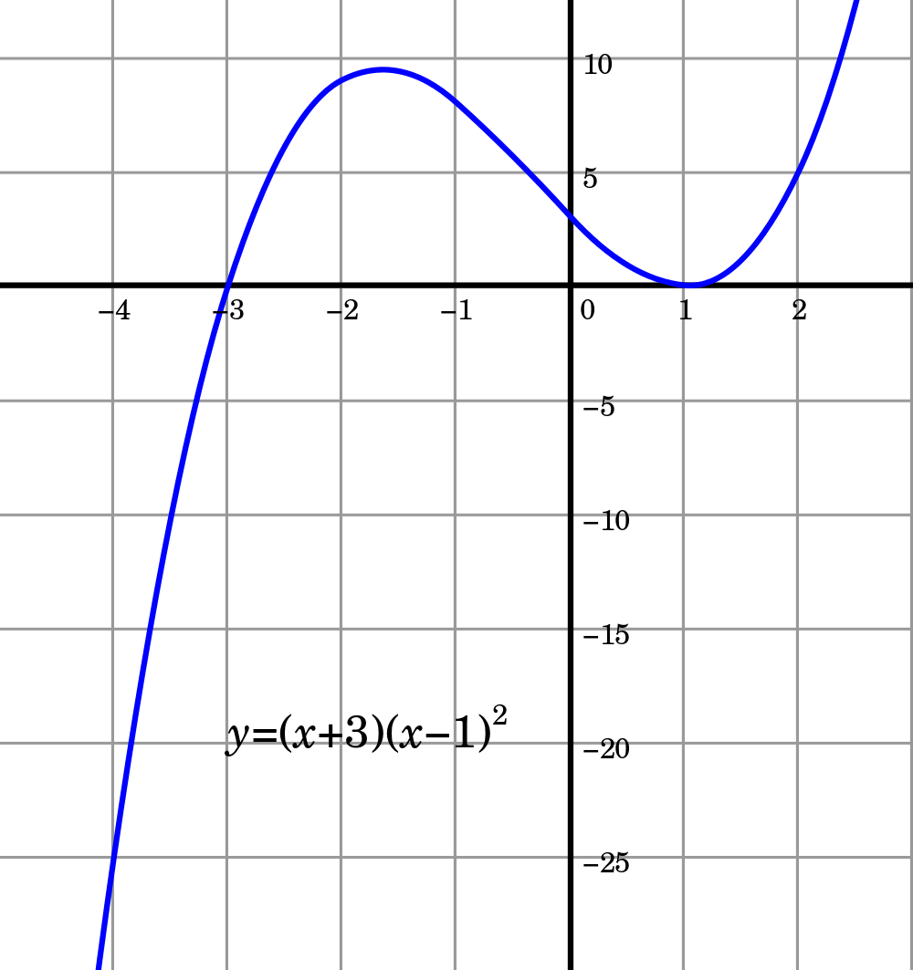
That’s not the kind of graph I mean.  I’m talking about the sort of object that’s studied in the field of graph theory, but which, confusingly, is more often referred to as a “network” outside that field.  Something like this:

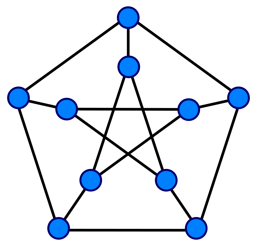
This is where the Tube Map comes in, because that’s a great example of a graph.  (You can click on the words “Tube Map” for a picture: I can’t show you a copy here because TfL charges licensing fees for use.)  There are “vertices” (singular “vertex”, as you may recall from GCSE Maths) or “nodes”, which are the stations in the Tube Map.  The vertices are joined by edges, which, in the case of the Tube Map, denote that you can go directly from the station at one end of the edge to the station at the other, without stopping at any stations in between.  (The Tube Map has additional features, like colours for the lines and symbols to denote interchanges and step-free access.  We don’t care about those in our mathematical graphs: all vertices are alike, and any edge from a vertex is like any other.)

The convention is to label the vertices with $1, 2, 3, \dotsc$, up to $n$, where $n$ is the number of vertices in the graph, and if we say “the graph on $n$ vertices” without further qualification, we’ll label the vertices in this way.  One more thing: you might ask if you can place an edge that starts and ends at the same vertex, or have more than one edge between a given pair of vertices.  Some people do say these are allowed in graphs—indeed, while there are no self-loops on the Tube Map, there are two edges between King’s Cross St Pancras and Euston, on the Northern and Victoria lines.  But we will assume neither of these things can be present in a true graph.  (With this convention, the objects that have self-loops and multiple edges are called “multigraphs”.)

The last thing from graph theory that we need to define is a “connected component” (or simply “component”).  We divide the graph into its components by saying that two vertices are in the same component if and only if you can get from one to the other by passing along edges of the graph.  For instance, on the Tube Map, there is only one component, because everything is ultimately connected to everything else.  The unofficial subway-style map of Amtrak shows two: most of the map is one component, but in the extreme north-east the Downeaster through Massachusetts, New Hampshire and Maine is not connected to anything else.  (At least, not via Amtrak services!) The maximum number of components in a graph, by contrast, is equal to the number of vertices; that case occurs when there are no edges at all, so each vertex forms its own component.

“But I thought your thesis was about probability?” I hear you ask.  We’re getting there.  We’ll be talking about random graphs for the rest of these posts.  A random graph is just a graph that’s chosen randomly.  More specifically, it’s common for the number of vertices to be picked, and graphs on those vertices to be chosen from some probability distribution.  It’s also possible to constrain still further to randomness within some structure, but we won’t be doing that here.

One of the simplest random graph models is called the Erdős–Rényi model, after two Hungarian mathematicians, Paul Erdős and Alfréd Rényi.  (Erdős in particular was a hugely prolific mathematician, and I could write a whole blog post about him.  In the meantime, check out his Wikipedia article.)  A simple example of it is this: take $n$ vertices, for whatever value of $n$ you choose.  Then take a fair coin (with probability $1/2$ of both heads and tails), and flip it repeatedly, once for every pair of vertices.  If it comes up heads on a flip, insert an edge between those two vertices.

But there’s no reason mathematically why the coin has to be fair.  Instead, we could do the same but let the probability of heads be $p$, for some $p$ between $0$ and $1$.  We will write this as $\mathcal{G}(n,p)$.  The crucial thing here is that the coin flips are independent: no flip affects any subsequent ones.  We’re also assuming that $n$ and $p$ are known: we’re leaving them as things we can choose however we please (within reason), but we’re not trying to infer from the graphs we see what the values of $n$ and $p$ are.  (This would be a valid question, but it would be a question of statistics rather than theoretical probability; that being said, the distinction is a little woolly.)

Hold on if you’re getting bogged down in the theory: we’re nearly at something rather spectacular, as mathematical results go.  Often a natural question when you have a value $n$ that has to be a positive whole number is: what happens when $n$ gets very large?  And so it is here.  It’s also natural, if you do this, to let $p$ depend on $n$, and an interesting choice to take is $p = \kappa/n$, for some value $\kappa$ (the Greek letter kappa), which can be any non-negative value: $1.5$, say, or $\pi$.  (You then have to make sure $n$ is big enough that $p$ is still between $0$ and $1$, but since we’re looking at what happens for very large $n$ that’s not a real problem.)

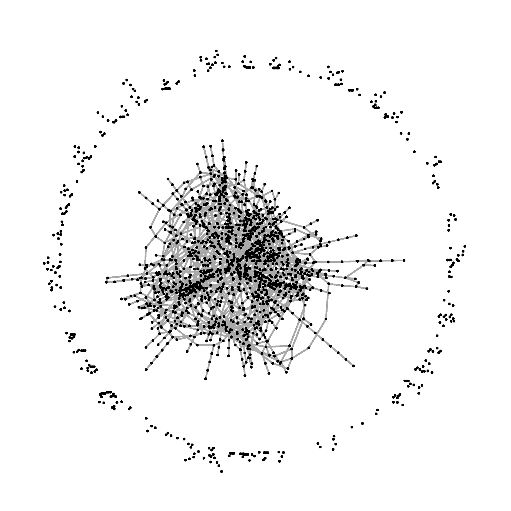
It turns out that you get dramatically different effects depending on whether $\kappa$ is bigger than or less than $1$.  If $\kappa$ is bigger than $1$, you usually get a large component (referred to as “the giant component”) and lots of smaller ones—in particular the largest one is roughly of size $cn$, where $c$ is some constant that depends on $\kappa$, and the others are much, much smaller.  Let’s look at a picture: here, we’re looking at the case of $\mathcal{G}(2000, 1/1000)$, so we’ve taken $\kappa=2$ with two thousand vertices. (Remember, this is a random graph, so it won’t in general look exactly like this. But it usually looks something like this.)

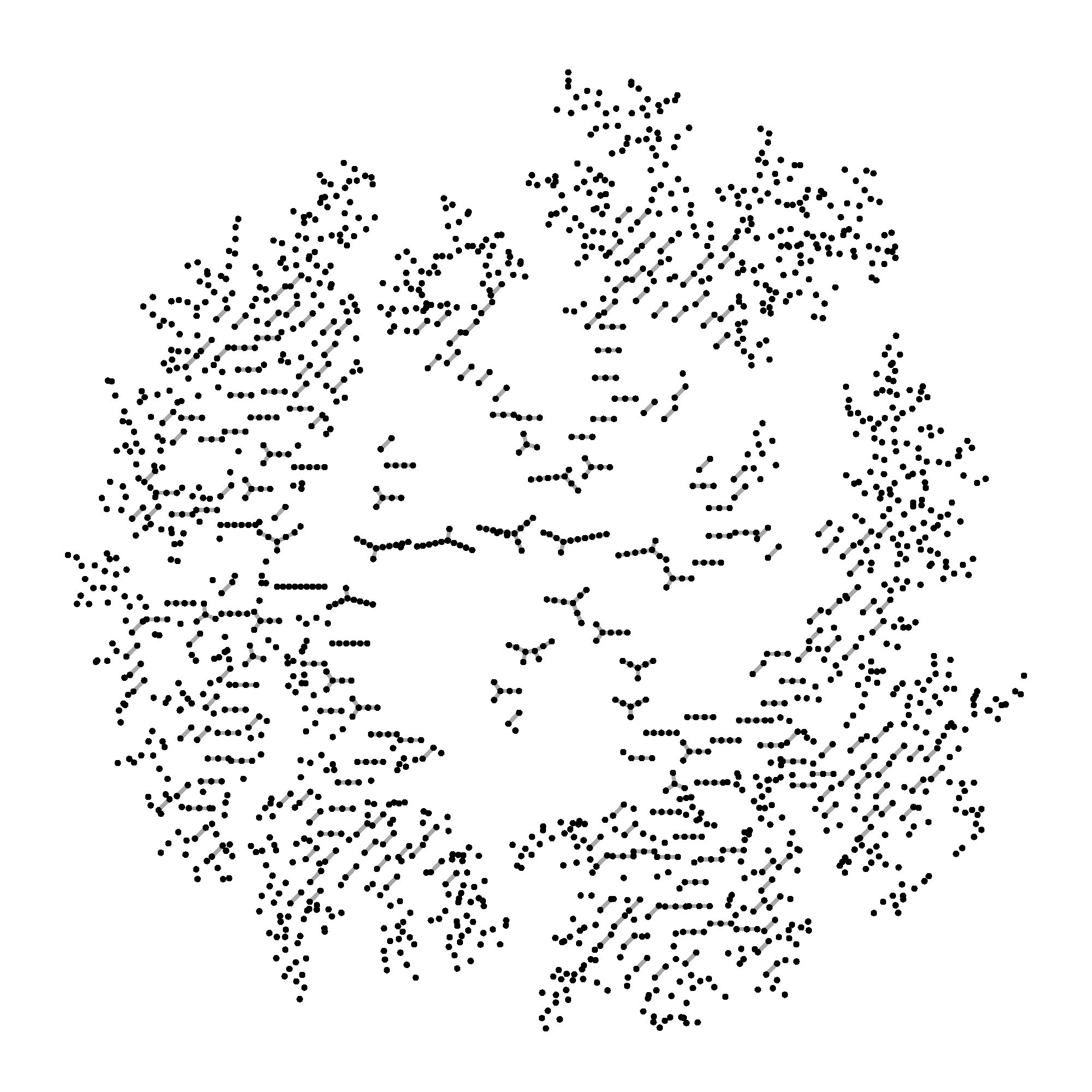
If $\kappa$ is less than $1$, you just get lots of tiny components, about the same size as the non-giant components in the other case.  Crucially, there’s no giant. (If you remember logarithms, the biggest component is roughly of size $d \log n$, where $d$ is a constant that depends on $\kappa$.) Here’s a picture again: here we’ve taken $\mathcal{G}(2000, 1/4000)$, so we still have two thousand vertices but now $\kappa = 1/2$.

This is a dramatic shift: if your $\kappa$ is at all less than $1$, even very slightly, you will see the small-component effect (for large enough $n$).  And even if your $\kappa$ is only a tiny bit bigger than $1$, you will eventually see the emergence of a giant.  That’s why it’s called a “phase transition”, by analogy with, say, what happens when you steadily apply heat to water—there’s no fundamental change in the structure of the substance until you reach 100°, at which point the form suddenly changes into a gas.

Why does this happen?  And what happens when $\kappa = 1$ exactly?  Well, this post is quite long enough, so those questions will have to wait until next time.